Next: 第15章 H25.2.27: 数値的に積分する Up: 応用理工学情報処理 Previous: 第13章 H25.2.13 ファイル処理 Contents Index
数学関数については, 「数学関数」[20.8.9] を参照のこと.
$ cc plot.c -lmまた, -Wall (Warning all)オプションを付けておくと, プログラム上の誤りがメッセージとして表示されるので効率よくプログラムを作成できる.
$ cc -Wall plot.c -lm
Tips:
例えば, 以下のようにより, emacs を終了しなくてもそのままその端末を使ってコンパイルすることができる.
$ emacs plot.c &
$ cc -Wall plot.c -lm
$ ./a.out
$ firefox drawing.svg &
ただし, ファイルを保存し忘れないように注意が必要である. firefox も &をつけてバックグラウンドで実行し, 端末と独立に実行した方が使いやすい.
$ cc -Wall plot.c -lm && ./a.outとすると, コンパイル(cc)に成功したときのみ, ./a.out が実行される.
成功か失敗かは, 実行したプログラム返した値が 0 か 0 でない数かで判断される. この値は, main 関数の return 文で返される値や 任意の行でプログラムを終了する関数であるexit関数の実引数の値が用いられる.
このセクションの最後にグラフをプロットするプログラムを掲載する. このプログラムを実行すると, SVG描画ファイル drawing.svg が作成され, これを表示すると下の図のようになる. main 関数中のパラメータを変えて表示してみると, 各パラメータの意味が掴みやすい.
![\includegraphics[width=15cm]{file/src/drawing.eps}](img62.png)
グラフでは, データのX座標Y座標の値でプロットされている. このデータの座標系を, ワールド座標系と呼ぶことにする. これは, 画面上の位置を表すスクリーン座標系とは異なる. 以降では, データの座標系をスクリーンの座標系に変換を行ってデータをプロットする.
データをプロットするためには, プロットする領域, すなわちx軸の初めと終わりの値, y軸の初めと終わりの値を指定してプロットする必要がある. これまでに挙げたプログラムではスクリーン座標系を用いた. この座標系では, yの値は下の方が大きくなるし, X軸, Y軸の縮尺は固定されている. そこで, データの値を表現する座標系(ワールド座標系)からスクリーン座標系に変換する plot_で始まる描画関数を用意した. plot_で始まる描画関数は, svg_で始まる描画関数と機能は全く同じであるが, plot_関数は, ワールド座標系の座標を受け取り, これをスクリーン座標に変換して, svg_で始まる同じ名前の関数に渡す. plot_関数を利用するために, 予め画面(スクリーン)描画する領域(ビュー)と, ワールド座標系を指定しておく必要がある.
下図で赤色で示された部分はワールド座標系を表し, 黒色で示された部分はスクリーン座標系を表す. 赤い四角内の座標をワールド座標系で表現し, これをスクリーン座標系に変換することにする.
![\includegraphics[width=15cm]{file/src/svg_36.eps}](img63.png)
下に, データのプロットを行うプログラムの例 (plot.c) を示す.
コンパイルの方法:
plot.c の中では, 描画に関係する部分は svg1.h というファイルに分割して記述し, 先頭の方の #include命令で取り込んでいる. #include は, その命令がある行に指定されたファイルの内容を展開する命令である. 前の章では svg0.h としたが, 混同しないように svg1.h とした. このようなファイルの分割については「ヘッダーファイルにする」[13.5.7]を参照のこと.
plot.c の内容:
#include <stdio.h>
#include <math.h>
#include "svg1.h"

int main(void)
{
	 SVG svg_file;
	 PLOT plot;
	 PLOT_VIEW view = {100.0, 50.0, 800.0, 500.0};
	 PLOT_WORLD world = {-1.0, -2.0, 21.0, 2.0};
	 PLOT_AXIS axis = {"X-Axis (unit)", 5, "Y-Axis (unit)", 5};
	 ATTRIBUTE circle_attrib   = {"blue", 1.0, "white"};
	 double x, y;

	 plot_file_open(&svg_file, "drawing.svg", 855.0, 605.0);
	 plot_init(&plot, &svg_file, &view, &world, &axis);

	 for(x=0.0; x<20.0; x+=0.1){
		  y = sin(x);
		  plot_circle_draw(&plot, x, y, 2.0, &circle_attrib);
	 }

	 plot_file_close(&plot);
	 return 0;
}
以下の内容を持つファイルを svg1.h として上のファイルと同じフォルダ/ディレクトリに保存. emacsでは, $ emacs svg1.h として新規ファイルを開き, この内容を書き込んだのち保存する. CPadでは新規ファイルを開いて, この内容を書き込みファイル名を指定して保存する.
#include <stdio.h>
#include <stdlib.h>
#include <math.h>

typedef struct {
	 FILE *fp;
	 double width, height;
} SVG;

typedef struct {
	 char *stroke;
	 double stroke_width;
	 char *fill;
	 double font_size;  // text: font size
	 char *text_anchor; // text: 位置合わせ "start", "middle", "end"
	 double dx, dy;     // text: テキストの基準位置(anchor)からのスクリーン座標系における位置補正
	 double rotation;   // text: 回転角度 (単位は度)
}  ATTRIBUTE;

typedef struct {
	 double x1, y1, x2, y2;
} PLOT_VIEW;

typedef struct {
	 double x1, y1, x2, y2;
} PLOT_WORLD;

typedef struct {
	 char *x_label;         // x 軸
	 int x_major_tics;      // 目盛線の数
	 char *y_label;         // y 軸
	 int y_major_tics;
} PLOT_AXIS;

typedef struct {
	 SVG *svg;
	 double sx, sy;
	 PLOT_VIEW v;
	 PLOT_WORLD w;
} PLOT;

/* ------------------------------------------------------------ */

// filename で指定されるファイルを開く.
// ファイルを開くことができない場合は, プログラムを終了する.
// SVG *svg の fp に開いたファイルのファイルポインタを代入する.
// width, height 画像の大きさ.
SVG *svg_open(SVG *svg, const char *filename, double width, double height)
{
	 svg->fp = fopen(filename, "w");
	 if(svg->fp==NULL){
		  printf("drawing.svg: File can not be created.");
		  exit(1);
	 }
	 fprintf(svg->fp,
			 "<?xml version=\"1.0\" encoding=\"UTF-8\" standalone=\"yes\"?>\n");
	 fprintf(svg->fp,
			 "<svg xmlns=\"http://www.w3.org/2000/svg\"\n"
			 " width=\"%g\" height=\"%g\" >\n", width, height);
	 svg->width = width;
	 svg->height = height;
	 return svg;
}

void svg_close(SVG *svg)
{
	 fprintf(svg->fp, "</svg>\n");
	 fclose(svg->fp);
}

/* ----------------------------------------------------------------------
   SVG描画関数
   svg_ で始まる関数は, スクリーン座標系に直接描画する.
   前回使用した関数と同一.
*/


void svg_line_draw(SVG *svg,
     double x1, double y1, double x2, double y2, const ATTRIBUTE *attrib)
{
	 fprintf(svg->fp,
			 "<line x1=\"%g\" y1=\"%g\" x2=\"%g\" y2=\"%g\"\n"
			 " stroke=\"%s\" stroke-width=\"%g\"/>\n",
			 x1, y1, x2, y2,  attrib->stroke, attrib->stroke_width);
}

void svg_rect_draw(SVG *svg,
     double width, double height, double x, double y, const ATTRIBUTE *attrib)
{
	 fprintf(svg->fp,
			 "<rect width=\"%g\" height=\"%g\" x=\"%g\" y=\"%g\" \n"
			 "stroke=\"%s\" stroke-width=\"%g\" fill=\"%s\" />\n",
			 width, height, x, y,
			 attrib->stroke, attrib->stroke_width, attrib->fill);
}

void svg_polyline_draw(SVG *svg,
     const double *x, const double *y, size_t n, const ATTRIBUTE *attrib)
{
	 size_t i;

	 fprintf(svg->fp, "<polyline points=\"");
	 for(i=0; i<n-1; i++)
		  fprintf(svg->fp, "%g %g,\n", x[i], y[i]);
	 fprintf(svg->fp, "%g %g\"\n", x[n-1], y[n-1]);
	 fprintf(svg->fp, "stroke=\"%s\" stroke-width=\"%g\" fill=\"%s\" />\n",
			 attrib->stroke, attrib->stroke_width, attrib->fill);
}

void svg_circle_draw(SVG *svg,
     double cx, double cy, double r, const ATTRIBUTE *attrib)
{
	 fprintf(svg->fp,
			 "<circle cx=\"%g\" cy=\"%g\" r=\"%g\"\n"
			 " stroke=\"%s\" stroke-width=\"%g\" fill=\"%s\" />\n",
			 cx, cy, r, attrib->stroke, attrib->stroke_width, attrib->fill);
}


void svg_text_draw(SVG *svg,
     double x, double y, const char *text, const ATTRIBUTE *attrib)
{
	 const double rotation_eps = 1.0e-16;
	 int i;
	 // 2010.2.10 修正 ここから
	 double rotation[4];
	 rotation[0] =  cos(attrib->rotation/180.0*M_PI);
	 rotation[1] = -sin(attrib->rotation/180.0*M_PI);
	 rotation[2] =  sin(attrib->rotation/180.0*M_PI);
	 rotation[3] =  cos(attrib->rotation/180.0*M_PI);
     // ここまで
	 for(i=0; i<4; i++){
		  if ( fabs(rotation[i]) < rotation_eps )
			   rotation[i] = 0.0;
	 }

	 fprintf(svg->fp,
			 "<text x=\"0\" y=\"0\"\n"
			 " font-size=\"%g\" text-anchor=\"%s\"\n"
			 " transform=\"matrix(%g, %g, %g, %g, %g, %g)\" >"
			 "%s</text>\n",
			 attrib->font_size, attrib->text_anchor,
			 rotation[0], rotation[1], rotation[2], rotation[3], x+attrib->dx, y+attrib->dy,
			 text);
}

/* ----------------------------------------------------------------------
   PLOT 描画関数
   plot_ で始まる関数は, ワールド座標系に描画する.
   ワールド座標系の座標を受け取り, 各関数の内部でスクリーン座標系に変換し,
   svg_ で始まる対応する関数を呼び出し, 描画する.
*/

// スクリーン座標系中で, 描画を行う領域ビューポートを指定する.
void plot_view_set(PLOT *plot, PLOT_VIEW *v)
{
	 plot->v.x1 = v->x1;
	 plot->v.y1 = v->y1;
	 plot->v.x2 = v->x2;
	 plot->v.y2 = v->y2;
}

// ビューポートにワールド座標系を設定する.
void plot_world_set(PLOT *plot, PLOT_WORLD *w)
{
	 plot->w.x1 = w->x1;
	 plot->w.y1 = w->y1;
	 plot->w.x2 = w->x2;
	 plot->w.y2 = w->y2;

	 plot->sx =  (plot->v.x2 - plot->v.x1) / (plot->w.x2 - plot->w.x1);
	 plot->sy =  (plot->v.y2 - plot->v.y1) / (plot->w.y2 - plot->w.y1);
}

// ワールド座標系のx座標を受け取り, スクリーン座標系のxに変換した値を返す.
double plot_wx2vx(PLOT *plot, double x)
{
	 return plot->v.x1 + plot->sx * (x - plot->w.x1);
}

// ワールド座標系のy座標を受け取り, スクリーン座標系のyに変換した値を返す.
double plot_wy2vy(PLOT *plot, double y)
{
	 return plot->v.y2 - plot->sy * (y - plot->w.y1);
}


void plot_line_draw(PLOT *plot,
    double x1, double y1, double x2, double y2, const ATTRIBUTE *attrib)
{
	 svg_line_draw(plot->svg,
				   plot_wx2vx(plot, x1), plot_wy2vy(plot, y1),
				   plot_wx2vx(plot, x2), plot_wy2vy(plot, y2),
				   attrib);
}

void ascending_order(double *a, double *b)
{
	 double tmp;
	 if(*a > *b){
		  tmp = *a;
		  *a = *b;
		  *b = tmp;
	 }
}

void plot_rect_draw(PLOT *plot,
     double width, double height, double x, double y, const ATTRIBUTE *attrib)
{
	 double vx1 = plot_wx2vx(plot, x), vx2 = plot_wx2vx(plot, x + width);
	 double vy1 = plot_wy2vy(plot, y), vy2 = plot_wy2vy(plot, y + height);
	 ascending_order(&vx1, &vx2);
	 ascending_order(&vy1, &vy2);
	 svg_rect_draw(plot->svg, vx2-vx1, vy2-vy1, vx1, vy1, attrib);
}

// 任意の大きさの配列を実行時に確保する.
// C99 では大きくない配列は より簡便に可変長配列により確保できる.
void *my_malloc(size_t n)
{
	 void *ptr = malloc(n);
	 if(ptr==NULL){
		  perror("my_malloc");
		  exit(1);
	 }
	 return ptr;
}

void plot_polyline_draw(PLOT *plot,
     const double *x, const double *y, size_t n, const ATTRIBUTE *attrib)
{
	 double *sx = (double *)my_malloc(sizeof(double)*n);
	 double *sy = (double *)my_malloc(sizeof(double)*n);
	 size_t i;

	 for(i=0; i<n; i++){
		  sx[i] = plot_wx2vx(plot, x[i]);
		  sy[i] = plot_wy2vy(plot, y[i]);
	 }
	 svg_polyline_draw(plot->svg, sx, sy, n, attrib);
	 free(sx);
	 free(sy);
}

void plot_circle_draw(PLOT *plot,
     double cx, double cy, double r, const ATTRIBUTE *attrib)
{
	 svg_circle_draw( plot->svg,
					  plot_wx2vx(plot, cx), plot_wy2vy(plot, cy), r, attrib);
}

void plot_text_draw(PLOT *plot,
     double x, double y, const char *text, const ATTRIBUTE *attrib)
{
	 svg_text_draw(plot->svg,
				   plot_wx2vx(plot, x), plot_wy2vy(plot, y), text, attrib);
}

/* ----------------------------------------------------------------------
   PLOT 関数
   PLOT描画関数を呼び出しグラフを作成するための関数.
*/

/*
  from から to を sect個にに分割した値をのうちきりのよい値を返す.
  これにより目盛を付ける座標を決める.
  prec: 返す値の桁数.
*/
double axis_tics_step_get(int *prec, double from, double to, int sect)
{
	 double delta, sign, factor, order;

	 delta = (to-from)/sect;

	 sign = (delta >= 0.0) ? 1.0 : -1.0;
	 delta = fabs(delta);

	 order = floor(log10(delta));

	 factor = delta / pow(10.0, order); // ここでは 1.0 <= delta < 10.0.
	 if(factor<2.0) // 1, 2, 5 の何れかに規格化
		  factor=1.0;
	 else if (factor<5.0)
		  factor = 2.0;
	 else
		  factor = 5.0;

	 *prec = ( order >= 0.0 ) ? 0 : -((int)order);
	 return sign * factor * pow(10.0, order);
}

// X軸の描画.
// 軸, 目盛, 目盛の数値, 軸の名前.
void plot_axis_x_linear_draw(PLOT *plot, PLOT_AXIS *axis, double y_base, double y_end,
     ATTRIBUTE *axis_attrib, ATTRIBUTE *tics_attrib, ATTRIBUTE *label_attrib)
{
	 int i;
	 char buff[128];
	 double p;     // 目盛の座標.
	 double step;  // 目盛の刻み幅.
	 int prec;     // 小数点以下の桁.

	 plot_line_draw(plot, plot->w.x1, y_base, plot->w.x2, y_base, axis_attrib);
	 step = axis_tics_step_get(&prec, plot->w.x1, plot->w.x2, axis->x_major_tics);
	 for(i=0; (p= ((int)(plot->w.x1*1.01/step)+i)*step) < plot->w.x2*1.01 ; i++){
		  snprintf(buff, sizeof(buff)/sizeof(char), "%.*f", prec, p);
		  plot_line_draw(plot, p, y_base, p, y_end, axis_attrib);
		  plot_text_draw(plot, p, y_base, buff, tics_attrib);
	 }
	 plot_text_draw(plot, (plot->w.x1 + plot->w.x2)/2.0, y_base, axis->x_label, label_attrib);
}

// Y軸の描画
void plot_axis_y_linear_draw(PLOT *plot, PLOT_AXIS *axis, double x_base, double x_edge,
     ATTRIBUTE *axis_attrib, ATTRIBUTE *tics_attrib, ATTRIBUTE *label_attrib)
{
	 int i;
	 char buff[128];
	 double p;     // 目盛の座標.
	 double step;  // 目盛の刻み幅.
	 int prec;     // 小数点以下の桁.

	 plot_line_draw(plot, x_base, plot->w.y1, x_base, plot->w.y2, axis_attrib);
	 step = axis_tics_step_get(&prec, plot->w.y1, plot->w.y2, axis->y_major_tics);
	 for(i=0; (p= ((int)(plot->w.y1*1.01/step)+i)*step) < plot->w.y2*1.01 ; i++){
		  snprintf(buff, sizeof(buff)/sizeof(char), "%.*f", prec, p);
		  plot_line_draw(plot, x_base, p, x_edge, p, axis_attrib);
		  plot_text_draw(plot, x_base, p, buff, tics_attrib);
	 }
	 plot_text_draw(plot, x_base, (plot->w.y2 + plot->w.y1)/2.0, axis->y_label, label_attrib);
}

// X軸とY軸の描画
void plot_axis_draw(PLOT *plot, PLOT_AXIS *axis)
{
	 ATTRIBUTE axis_attrib = {"black",  1.0, "none",   0.0};
	 ATTRIBUTE x_tics_attrib     = {"black", 0.0, "green", 15.0, "middle",  0.0,  20.0,  0.0};
	 ATTRIBUTE x_label_attrib    = {"black", 0.0, "green", 15.0, "middle",  0.0,  50.0,  0.0};
	 ATTRIBUTE y_tics_attrib     = {"black", 0.0, "green", 15.0, "end",    -5.0,   6.0,  0.0};
	 ATTRIBUTE y_label_attrib    = {"black", 0.0, "green", 15.0, "middle",-50.0,   0.0, 90.0};

	 double x_base, x_edge, y_base, y_edge;

	 // x-axis
	 y_base = plot->w.y1;
	 y_edge = y_base + 0.02*(plot->w.y2-y_base);
	 plot_axis_x_linear_draw(plot, axis, y_base, y_edge, &axis_attrib, &x_tics_attrib, &x_label_attrib);

	 // y-axis
	 x_base = plot->w.x1;
	 x_edge = plot->w.x1 + 0.02*(plot->w.x2 - plot->w.x1);
	 plot_axis_y_linear_draw(plot, axis, x_base, x_edge, &axis_attrib, &y_tics_attrib, &y_label_attrib);
}


// PLOT の初期化.
PLOT *plot_init(PLOT *plot, SVG *svg, PLOT_VIEW *v, PLOT_WORLD *w, PLOT_AXIS *axis)
{
	 ATTRIBUTE background_attrib = {"none",  1.0, "white",  0.0};
	 plot->svg = svg;
	 plot_view_set(plot, v);
	 plot_world_set(plot, w);
	 plot_rect_draw(plot, w->x2 - w->x1, w->y2 - w->y1, w->x1, w->y1, &background_attrib);
	 plot_axis_draw(plot, axis);

	 return plot;
}

// 描画ファイルを開く.
SVG *plot_file_open(SVG *svg, char *filename, double width, double height)
{
	 static ATTRIBUTE background_attrib = {"none",  1.0, "cornsilk",  0.0};
	 svg_open(svg, filename, width, height);
	 svg_rect_draw(svg, width, height, 0.0, 0.0, &background_attrib);
	 return svg;
}

// 描画ファイルを閉じる.
void plot_file_close(PLOT *plot)
{
	 svg_close(plot->svg);
}
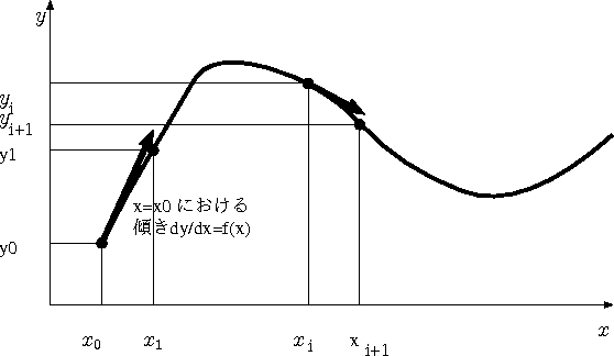
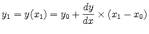
微分方程式
図5に示すように, ![]() から微小量離れた
から微小量離れた ![]() における
における
![]() の関数値を求めることを考える.
の関数値を求めることを考える. ![]() における傾き
における傾き
![]() は,
は,
![]() と与えられている. 従って, 近似的に
と与えられている. 従って, 近似的に
ここでは,具体的な例として微分方程式
| (8) |
![]() ,
, ![]() ,
,
 から
から
![]() を求めるプログラムは次のようになる. ただし今後のため
を求めるプログラムは次のようになる. ただし今後のため ![]() と定義した.
と定義した.
#include <stdio.h>
#include <math.h>

/*
    dy/dx = cos(x)
    x0 = 0.0
    y0 = 1.0
*/

double f(double x)
{
  double fx;

  fx = cos(x);

  return fx;
}

int main(void)
{
  double h;
  double x0, x1;
  double y0, y1;

  x0 = 0.0;
  h = 0.25;
  y0 = 1.0;
  printf("%g %g\n",  x0, y0);

  x1 = x0 + h;
  y1 = y0 + f(x0) * h;
  printf("%g %g\n",  x1, y1);

  return 0;
}
図5 に示すように, 一般に ![]() 番目の
番目の ![]() ,
, ![]() から
から
![]() ,
, ![]() を求めることができる. このときには
を求めることができる. このときには
#include <stdio.h>
#include <math.h>

double f(double x)
{
  double fx;

  fx = cos(x);

  return fx;
}

int main(void)
{
  double h;
  double x0, x1, x2, x3, x4, x5, x6, x7, x8, x9, x10;
  double y0, y1, y2, y3, y4, y5, y6, y7, y8, y9, y10;

  x0 = 0.0;
  h = 0.25;
  y0 = 1.0;
  printf("%g %g\n",  x0, y0);

  x1 = x0 + h;
  y1 = y0 + f(x0) * h;
  printf("%g %g\n",  x1, y1);

  x2 = x1 + h;
  y2 = y1 + f(x1) * h;
  printf("%g %g\n",  x2, y2);

  x3 = x2 + h;
  y3 = y2 + f(x2) * h;
  printf("%g %g\n",  x3, y3);

  x4 = x3 + h;
  y4 = y3 + f(x3) * h;
  printf("%g %g\n",  x4, y4);

  x5 = x4 + h;
  y5 = y4 + f(x4) * h;
  printf("%g %g\n",  x5, y5);

  x6 = x5 + h;
  y6 = y5 + f(x5) * h;
  printf("%g %g\n",  x6, y6);

  x7 = x6 + h;
  y7 = y6 + f(x6) * h;
  printf("%g %g\n",  x7, y7);

  x8 = x7 + h;
  y8 = y7 + f(x7) * h;
  printf("%g %g\n",  x8, y8);

  x9 = x8 + h;
  y9 = y8 + f(x8) * h;
  printf("%g %g\n",  x9, y9);

  x10 = x9 + h;
  y10 = y9 + f(x9) * h;
  printf("%g %g\n",  x10, y10);

  return 0;
}
10 回も同じことを書くのは面倒であるし, 100回を越えるとプログラム
のサイズも無駄に大きくなる.
同じことを繰り返している部分を for を用いて表現すると下のようになる.
分割数 ![]() を大きくすることで 刻み幅
を大きくすることで 刻み幅 ![]() を小さくすると誤差はどのように変
化するか調べよ.
を小さくすると誤差はどのように変
化するか調べよ.
#include <stdio.h>
#include <math.h>

double f(double x)
{
  double fx;

  fx = cos(x);

  return fx;
}

int main(void)
{
  int i, n;
  double h;
  double x, x0, x1, y;

  x0 = 0.0;
  x1 = 2.5;
  n = 10;

  x = x0;
  h = (x1-x0)/n;
  y = 1.0;
  printf("%g %g\n",  x, y);

  for(i=0; i<n; i++){
    y = y + f(x) * h;
    x = x + h;
    printf("%g %g\n",  x, y);
  }

  return 0;
}
![\includegraphics[width=15cm]{numerical/euler1.eps}](img94.png)
inkscape で SVGファイルを開く場合は,
$ inkscape & もしくは $ inkscapeのように 一度コマンドラインから起動し,
「ファイル」![]() 「開く」によりファイルを指定してSVGファイルを開く.
「開く」によりファイルを指定してSVGファイルを開く.
通常 $ inkscape drawing.svg のようにファイル名を指定して起動できますが, 全学計算機システムでは設定が十分されていないようです.
svg1.h を用意したフォルダ/ディレクトリに以下のプログラム(.cが付くファイル)を作成して実行すると, グラフが plot_file_open 関数で指定したファイル(.svgが付くファイル)に出力される.
#include <stdio.h>
#include <math.h>
#include "svg1.h"

double f(double x)
{
  double fx;

  fx = cos(x);

  return fx;
}

int main(void)
{
	 // プロットに関係する変数.
	 SVG svg_file;
	 PLOT plot;
	 PLOT_VIEW view = {100.0, 50.0, 800.0, 500.0};
	 PLOT_WORLD world = {-1.0, 0.5, 21.0, 3.0};
	 PLOT_AXIS axis = {"x", 5, "y", 5};
	 ATTRIBUTE circle_attrib   = {"blue", 1.0, "white"};

	 // 数値計算に関係する変数.
	 int i;
	 double x, y;
	 int n;         // 分割数
	 double h;      // 刻み幅
	 double x0, x1; // x=x0 から x=x1 の範囲で解く.

	 // プロット初期化
	 plot_file_open(&svg_file, "drawing.svg", 855.0, 605.0);
	 plot_init(&plot, &svg_file, &view, &world, &axis);

	 // 数値計算
	 x0 = 0.0;
	 x1 = 2.5;
	 n = 10;

	 x = x0;
	 h = (x1-x0)/n;
	 y = 1.0;
	 //printf("%g %g\n",  x, y);
	 plot_circle_draw(&plot, x, y, 2.0, &circle_attrib);

	 for(i=0; i<n; i++){
		  y = y + f(x) * h;
		  x = x + h;
		  // printf("%g %g\n",  x, y);
		  plot_circle_draw(&plot, x, y, 2.0, &circle_attrib);
	 }

	 // プロット終了
	 plot_file_close(&plot);
	 return 0;
}
先に示した例では, 解析解が ![]() であることが分かっている.
こそで下に, 得られた数値解
であることが分かっている.
こそで下に, 得られた数値解![]() (赤)と解析解(青)を同時にプロットして比較してみた.
また誤差として両者の差
(赤)と解析解(青)を同時にプロットして比較してみた.
また誤差として両者の差
![]() (緑)もプロットしてある.
(緑)もプロットしてある.
![\includegraphics[width=15cm]{numerical/euler3.eps}](img98.png)
PLOT_WORLD 構造体の world の初期化の部分を変更すると, 表示される領域を広くしたり狭くしたりできることに注意. これまでと同様に, svg1.h を作成したフォルダ/ディレクトリに以下のプログラム(.cが付くファイル)を作成し, コンパイルする.
#include <stdio.h>
#include <math.h>
#include "svg1.h"

double f(double x)
{
	 double fx;

	 fx = cos(x);

	 return fx;
}

int main(void)
{
	 SVG svg_file;
	 PLOT plot;
	 PLOT_VIEW view = {100.0, 50.0, 800.0, 500.0};
	 PLOT_WORLD world = {-1.0, -0.5, 110.0, 2.5};
	 PLOT_AXIS axis = {"X", 5, "Y", 5};
	 ATTRIBUTE analytical_value = {"blue", 1.0, "none"};
	 ATTRIBUTE numerical_value  = {"red" , 1.0, "none"};
	 ATTRIBUTE error            = {"green" , 1.0, "white"};

	 int i, n;
	 double h;
	 double x, x0, x1, y;

	 // プロット初期化
	 plot_file_open(&svg_file, "drawing.svg", 855.0, 605.0);
	 plot_init(&plot, &svg_file, &view, &world, &axis);

	 // 数値計算
	 x0 = 0.0;
	 x1 = 100.0;
	 n = 1000;

	 x = x0;
	 h = (x1-x0)/n;
	 y = 1.0;
	 //printf("%g %g\n",  x, y);
	 plot_circle_draw(&plot, x, y, 1.0, &numerical_value);
	 plot_circle_draw(&plot, x, 1.0+sin(x), 1.0, &analytical_value);

	 for(i=0; i<n; i++){
		  y = y + f(x) * h;
		  x = x + h;
		  // printf("%g %g\n",  x, y);
		  plot_circle_draw(&plot, x, y, 1.0, &numerical_value);
		  plot_circle_draw(&plot, x, 1.0+sin(x), 1.0, &analytical_value);
		  plot_circle_draw(&plot, x, (1.0+sin(x)-y), 1.0, &error);
	 }


	 // プロット終了
	 plot_file_close(&plot);

	 return 0;
}
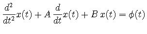
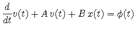
高階の常微分方程式も同様にEuler法により数値的に解ける。
馴染みのある例として質点が外力を受け位置![]() が時間と共に変化するような場
合を考える. このとき,
が時間と共に変化するような場
合を考える. このとき, ![]() に対する微分方程式は次のようになる.
に対する微分方程式は次のようになる.
 |
(10) |
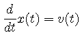
ここで, ![]() の他に速度
の他に速度![]() を導入する.
ここで,
を導入する.
ここで,
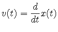 である.
である.
このとき, 上の式は,
 |
(11) |
 |
(12) | ||
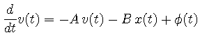 |
(13) |
このように2階偏微分方程式は
 |
(14) | ||
 |
(15) |
 |
(16) | ||
 |
(17) |
ここで
![]() ,
,
![]() であることに注意すると,
であることに注意すると,
 |
(18) | ||
 |
(19) |
| (20) | |||
| (21) |
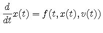
![]() を一定の値dtに固定する. また,
を一定の値dtに固定する. また, ![]() をx,
をx, ![]() をv,
をv,
![]() をt と表すことにすると, C言語では以下のようになる.
をt と表すことにすると, C言語では以下のようになる.
x = x + f(t, x, v) * dt;
v = v + g(t, x, v) * dt;
より簡潔に
x += f(t, x, v) * dt;
v += g(t, x, v) * dt;
と表すことができる.
 |
(22) |
 により
により  |
(23) | ||
 |
(24) |
| (25) | |||
 |
(26) |
さらに, 微小な角度でしか振動しない場合,
![]() と近似する場合もある.
このとき
と近似する場合もある.
このとき
| (27) | |||
 |
(28) |
 である.
このプログラムでは, 時刻
である.
このプログラムでは, 時刻
#include <stdio.h>
#include <math.h>

double L=1.0;        /* [m] */
double G = 9.80665;  /* [m/s^2] */

double f(double t, double theta, double omega)
{
	 return omega;
}

double g(double t, double theta, double omega)
{
	 return - G / L * theta;
}

int main(void)
{
	 int n = 1000;                    // 分割数
	 double t, t0=0.0, t1=5.0;        // [t0, t1]の範囲で解く.
	 double theta0 =80.0/180.0*M_PI;  // 初期値: theta = 80度
	 double omega0=0.0;               // 初期値: omega = 0

	 double theta = theta0, omega = omega0;
	 double dt = (t1-t0)/(double)n;

	 printf("%g %g %g %g\n", t, theta, omega, theta);

	 for(t=t0; t<=t1; t+=dt){
		  theta += f(t, theta, omega) * dt;
		  omega += g(t, theta, omega) * dt;
		  printf("%f %f %f %f\n", t, theta, omega, theta0*cos(sqrt(G/L)*t));
	 }

	 return 0;
}
プロットすると次のようになる. 予め svg1.h [14.3] をこのプログラムと同じフォルダ/ディレクトリに作成しておくこと.
#include <stdio.h>
#include <math.h>
#include "svg1.h"


double L=1.0;        /* [m] */
double G = 9.80665;  /* [m/s^2] */

double f(double t, double theta, double omega)
{
	 return omega;
}

double g(double t, double theta, double omega)
{
	 return - G / L * theta;
}

int main(void)
{
	 // プロット
	 SVG svg_file;
	 PLOT plot;
	 PLOT_VIEW view = {100.0, 50.0, 800.0, 500.0};
	 PLOT_WORLD world = {-1.0, -2.0, 6.0, 2.0};
	 PLOT_AXIS axis = {"t", 5, "theta", 5};
	 ATTRIBUTE analytical_value = {"blue", 1.0, "none"};
	 ATTRIBUTE numerical_value  = {"red" , 1.0, "none"};

	 // 数値計算
	 int n = 1000;                    // 分割数
	 double t, t0=0.0, t1=5.0;        // [t0, t1]の範囲で解く.
	 double theta0 =80.0/180.0*M_PI;  // 初期値: theta = 80度
	 double omega0=0.0;               // 初期値: omega = 0

	 double theta = theta0, omega = omega0;
	 double dt = (t1-t0)/(double)n;

	 // プロット初期化
	 plot_file_open(&svg_file, "drawing.svg", 855.0, 605.0);
	 plot_init(&plot, &svg_file, &view, &world, &axis);

	 printf("%g %g %g %g\n", t, theta, omega, theta);

	 for(t=t0; t<=t1; t+=dt){
		  theta += f(t, theta, omega) * dt;
		  omega += g(t, theta, omega) * dt;
		  // printf("%f %f %f %f\n", t, theta, omega, theta0*cos(sqrt(G/L)*t));
		  plot_circle_draw(&plot, t, theta, 1.0, &numerical_value);
		  plot_circle_draw(&plot, t, theta0*cos(sqrt(G/L)*t), 1.0, &analytical_value);

	 }

	 // プロット終了
	 plot_file_close(&plot);

	 return 0;
}
解析解(青)と数値解(赤)が重なって, 同じ結果が得られたことが分かる.
![\includegraphics[width=15cm]{numerical/Euler2ndOrderA1.eps}](img139.png)
上の例では,
![]() と近似した.
次にこの近似を用いずに数値解を求めてみる. このとき, Euler法による近似は次のようになる.
と近似した.
次にこの近似を用いずに数値解を求めてみる. このとき, Euler法による近似は次のようになる.
| (29) | |||
|
(30) |
#include <stdio.h>
#include <math.h>
#include "svg1.h"


double L=1.0;        /* [m] */
double G = 9.80665;  /* [m/s^2] */

double f(double t, double theta, double omega)
{
	 return omega;
}

double g(double t, double theta, double omega)
{
	 return - G / L * sin(theta);
}

int main(void)
{
	 // プロット
	 SVG svg_file;
	 PLOT plot;
	 PLOT_VIEW view = {100.0, 50.0, 800.0, 500.0};
	 PLOT_WORLD world = {-1.0, -2.0, 6.0, 2.0};
	 PLOT_AXIS axis = {"t", 5, "theta", 5};
	 ATTRIBUTE analytical_value = {"blue", 1.0, "none"};
	 ATTRIBUTE numerical_value  = {"red" , 1.0, "none"};

	 // 数値計算
	 int n = 1000;                    // 分割数
	 double t, t0=0.0, t1=5.0;        // [t0, t1]の範囲で解く.
	 double theta0 =80.0/180.0*M_PI;  // 初期値: theta = 80度
	 double omega0=0.0;               // 初期値: omega = 0

	 double theta = theta0, omega = omega0;
	 double dt = (t1-t0)/(double)n;

	 // プロット初期化
	 plot_file_open(&svg_file, "drawing.svg", 855.0, 605.0);
	 plot_init(&plot, &svg_file, &view, &world, &axis);

	 printf("%g %g %g %g\n", t, theta, omega, theta);

	 for(t=t0; t<=t1; t+=dt){
		  theta += f(t, theta, omega) * dt;
		  omega += g(t, theta, omega) * dt;
		  // printf("%f %f %f %f\n", t, theta, omega, theta0*cos(sqrt(G/L)*t));
		  plot_circle_draw(&plot, t, theta, 1.0, &numerical_value);
		  plot_circle_draw(&plot, t, theta0*cos(sqrt(G/L)*t), 1.0, &analytical_value);

	 }

	 // プロット終了
	 plot_file_close(&plot);

	 return 0;
}
この例では,
![]() で静かに離したのちの振り子の角度
で静かに離したのちの振り子の角度![]() を求めている.
このように
を求めている.
このように![]() が大きい場合には,
が大きい場合には,
![]() の近似は成り立たないことが分かる.
の近似は成り立たないことが分かる.
![\includegraphics[width=15cm]{numerical/Euler2ndOrderA2.eps}](img140.png)
※数学的には, 振り子の厳密解は楕円積分を用いて表される.
振り子の例で分かるように, 解析的な解を得るためには, 近似をしなければならない場合があるが, 数値解を求めるためにはそのような近似をしなくても解くことができ, より真の解に近い解を得ることができる可能性がある.
強制振動は変位![]() が
が
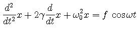 |
(31) |
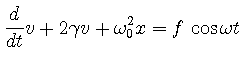
 を導入すると
 |
(32) | ||
 |
(33) |
 |
(34) | ||
 |
(35) |
| (36) | |||
| (37) |
x += v * dt;
v += (-2.0*gamma*v - omega0*omega0*x + f*cos(omega*t)) * dt;
と記述できる. 以下に強制振動を解くプログラムを挙げる.
#include <stdio.h>
#include <math.h>

double f(double t, double x, double v)
{
	 return v;
}

double g(double t, double x, double v)
{
	 double gamma = 0.5;
	 double omega0 = 10.0;
	 double f = 0.2;
	 double omega = 13.0;
	 return  -2.0*gamma*v - omega0*omega0*x + f*cos(omega*t);
}

int main(void)
{
	 int n = 1000;
	 double t, t0=0.0, t1=10.0;
	 double dt = (t1-t0)/(double)n;
	 double x = 0.0, v=1.0;

	 printf("%f %f %f\n", t, x, v);

	 for(t=t0; t<=t1; t+=dt){
		  x += f(t, x, v) * dt;
		  v += g(t, x, v) * dt;
		  printf("%f %f %f\n", t, x, v);
	 }

	 return 0;
}
この例のように解析解を求めるのが煩雑な場合でも,数値計算では容易に解が得られる. ただし, 各パラメータを変化させて, 解にどのような影響を及ぼしているか調べ, 物理的な描像を描くことが重要である.
(c)1999-2013 Tetsuya Makimura