Next: 第16章 H24.2.29: データ, 配列, Up: 応用理工学情報処理 Previous: 第14章 H25.2.20 数値計算: 微分方程式を解く Contents Index
積分領域を微小領域に区切り, 各領域で被積分関数![]() を多項式で近似することで,
数値的に積分値を求めることができる.
を多項式で近似することで,
数値的に積分値を求めることができる.
最後に, 以下の自分で作成, 実行した結果をメールで送る.
【注意】
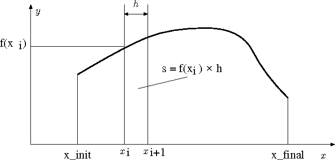
定積分を数値的に求める.
そこでまず, 積分区間を分割し, 各区間の面積を長方形の面積で近似する.
これは積分区間
![]() の関数
の関数![]() の値を,
一定の値
の値を,
一定の値![]() で近似することを意味する.
すなわち各区間内の関数
で近似することを意味する.
すなわち各区間内の関数![]() の値は0次式で近似されていることになる.
の値は0次式で近似されていることになる.
定積分
図6に示すように積分区間 [x_init, x_final] を ![]() 分割する.
分割する. ![]() 番目の区間で決まる部分の面積
番目の区間で決まる部分の面積 ![]() は 近似的に
は 近似的に
![]() で表される.
で表される.
具体的な例として定積分
#include <stdio.h>
#include <math.h>

double f(double x)
{
  double fx;

  fx = cos(x);
  return fx;
}

int main(void)
{
  int n;
  double x_init, x_final, h;
  double x0, x1, x2, x3, x4, x5, x6, x7, x8, x9;
  double s;

  x_init = 0.0;
  x_final = 1.0;
  n = 10;

  h = (x_final - x_init) / n;
  x0 = x_init;
  s = 0.0;

  s = s + f(x0) * h;

  x1 = x0 + h;
  s = s + f(x1) * h;

  x2 = x1 + h;
  s = s + f(x2) * h;

  x3 = x2 + h;
  s = s + f(x3) * h;

  x4 = x3 + h;
  s = s + f(x4) * h;

  x5 = x4 + h;
  s = s + f(x5) * h;

  x6 = x5 + h;
  s = s + f(x6) * h;

  x7 = x6 + h;
  s = s + f(x7) * h;

  x8 = x7 + h;
  s = s + f(x8) * h;

  x9 = x8 + h;
  s = s + f(x9) * h;

  printf("%g, %g\n", s, sin(1.0));

  return 0;
}
for を使って下のように簡潔に表現できる.
分割数 ![]() を大きくすると刻み幅
を大きくすると刻み幅 ![]() が小さくなる.
このとき誤差はどのようになるか調べよ.
が小さくなる.
このとき誤差はどのようになるか調べよ.
#include <stdio.h>
#include <math.h>

double f(double x)
{
  double fx;

  fx = cos(x);
  return fx;
}

int main(void)
{
  int i, n;
  double x_init, x_final, x, h;
  double s;

  x_init = 0.0;
  x_final = 1.0;
  n = 10;

  h = (x_final - x_init) / n;
  x = x_init;
  s = 0;

  for(i=0; i<n; i++){
    s = s + f(x) * h;
    x = x + h;
  }

  printf("numerical value: %g, analytical value: %g\n", s, sin(1.0));

  return 0;
}
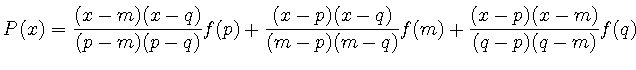
区間
![]() における関数
における関数![]() の値を,
点
の値を,
点![]() と 点
と 点
![]() を通る直線で近似すると,
より精度の高い近似となる.
を通る直線で近似すると,
より精度の高い近似となる.
このとき面積![]() は,
は,
ただし各区間の長さ(すなわち台形の底辺の長さ)を
![]() とした.
とした.
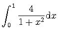
例として,
![$\textstyle \displaystyle \int_0^1 \frac{4}{1+x^2} \mathrm{d} x = [\arctan x]{}_0^1 = \pi$](img166.png) |
(40) |
#include <stdio.h>
#include <math.h>

/* Eqn (5.7) in p. 112. */

double func(double x)
{
	 double ret;

	 ret = 4.0/(1.0+x*x);
	 return ret;
}

double daikei(double x0, double xn, int n)
{
	 int i;
	 double y0 = func(x0);
	 double yn = func(xn);
	 double h = (xn - x0) / n;
	 double sum = 0.0;
	 double yi, xi;

	 sum = (y0 + yn)/2.0;

	 for(i=1; i<n; i++){
		  xi = x0 + h*i;
		  yi = func(xi);
		  sum += yi;
	 }
	 return sum * h;
}

int main(void)
{
	 double I;

	 I = daikei(0.0, 1.0, 10);
	 printf("daikei: I=%g\n", I);

	 return 0;
}
分割数を増やすと誤差がどのように変化するか調べてみる.
この場合, 解析解(analytical_value=![]() )が分かっているので,
数値解(numerical_value)の誤差は
)が分かっているので,
数値解(numerical_value)の誤差は ![]() - numerical_value である.
この値は何桁も変化するので,
- numerical_value である.
この値は何桁も変化するので,
![]() の値をプロットすることにする.
この値は何桁目まで正しいかを表している.
たとえば n=4000のとき誤差は
の値をプロットすることにする.
この値は何桁目まで正しいかを表している.
たとえば n=4000のとき誤差は![]() の程度である.
ただし, 一般にはanalytical_value - numerical_value
は負の値になる場合もあるので, エラーにならないように,
実数の絶対値を返すfabs関数により,
log10関数の引数を常に正になるようにしている.
の程度である.
ただし, 一般にはanalytical_value - numerical_value
は負の値になる場合もあるので, エラーにならないように,
実数の絶対値を返すfabs関数により,
log10関数の引数を常に正になるようにしている.
また, M_PIは 環境によっては math.hの中で有効桁の範囲で円周率![]() に定義されている. 定義されていない場合は次のように自分で定義しておく必要がする.
に定義されている. 定義されていない場合は次のように自分で定義しておく必要がする.
#define M_PI 3.14
#include <stdio.h>
#include <math.h>
#include "svg1.h"


double func(double x)
{
    double ret;

    ret = 4.0/(1.0+x*x);
    return ret;
}

double daikei(double x0, double xn, int n)
{
    int i;
    double y0 = func(x0);
    double yn = func(xn);
    double h = (xn - x0) / n;
    double sum = 0.0;
    double yi, xi;

    sum = (y0 + yn)/2.0;

    for(i=1; i<n; i++){
	xi = x0 + h*i;
	yi = func(xi);
	sum += yi;
    }
    return sum * h;
}

int main(void)
{
    int n; // 分割数

    // プロットに関係する変数.
    SVG svg_file;
    PLOT plot;
    PLOT_VIEW view = {100.0, 50.0, 800.0, 500.0};
    PLOT_WORLD world = {0.0, -10.0, 10000.0, 0.1};
    PLOT_AXIS axis = {"n", 5, "log10(error) = log10(M_PI - I)", 5};
    ATTRIBUTE circle_attrib   = {"blue", 1.0, "white"};

    // 数値計算に関係する変数.
    double analytical_value; // 解析解 (数学的に得られた値)
    double numerical_value;  // 数値解 (数値計算により得られた値)
    double error_order;      // 数値解の誤差の桁 (何桁目まで正しいかを表す指標)

    // プロット初期化
    plot_file_open(&svg_file, "drawing.svg", 855.0, 605.0);
    plot_init(&plot, &svg_file, &view, &world, &axis);

    // 分割数を変えて積分を数値的に求める.
    for(n=10; n<10000; n+=100){
	numerical_value = daikei(0.0, 1.0, n);
	analytical_value = M_PI;
	error_order = log10( fabs( numerical_value - analytical_value) );
	// printf("daikei: I=%g\n", error_order);
	plot_circle_draw(&plot, n, error_order, 2.0, &circle_attrib);
    }

    // プロット終了
    plot_file_close(&plot);

    return 0;
}
実行結果:
![\includegraphics[width=15cm]{numerical/daikeiB0.eps}](img169.png)
 |
(41) |
 は
は
 |
(42) | ||
 |
(43) | ||
 |
(44) | ||
 |
(45) | ||
 |
(46) | ||
 |
(47) |
例として,
|
(48) |
#include <stdio.h>
#include <math.h>

double func(double x)
{
  double ret;
  ret = 4.0/(1.0+x*x);
  return ret;
}

double Simpson(double x_0, double x_2n, int n)
{
	 double h = (x_2n - x_0) / (2.0*n);
	 double sum = 0.0;
	 int j;
	 double x_2j, x_2j1, y_2j, y_2j1;

	 sum  = h/3.0* func(x_0);

	 for(j=1; j<=n; j++){
		  x_2j1 = x_0 + (2*j-1)*h;
		  y_2j1 = func(x_2j1);
		  sum += h/3.0*4.0*y_2j1;
	 }

	 for(j=1; j<n; j++){
		  x_2j = x_0 + 2*j*h;
		  y_2j = func(x_2j);
		  sum += h/3.0*2.0*y_2j;
	 }

	 sum += h/3.0* func(x_2n);

	 return sum;
}

int main(void)
{
	 double I;

	 I = Simpson(0.0, 1.0, 5);
	 printf("Simpson: I=%g\n", I);

	 return 0;
}
台形公式(![]() )とシンプソンの公式(
)とシンプソンの公式(![]() )を比較してみる.
)を比較してみる.
 |
(49) | ||
 |
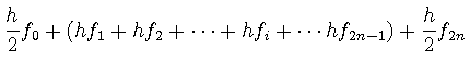
(50) |
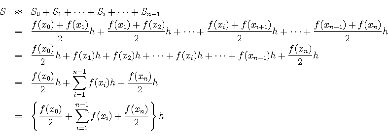
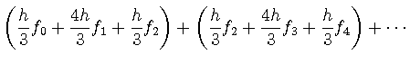
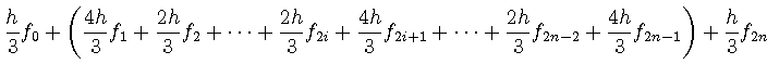
台形公式では, 一定の重みで加えているのに対し,
シンプソンの公式では, 隣接する組を
 の重みを付けて足し合わせている点が異なる.
以下のプログラムでは, 台形法とシンプソン法により積分
 の値を求め,
解析解との差を 対数をとってから表示している.
の値を求め,
解析解との差を 対数をとってから表示している.
#include <stdio.h>
#include <math.h>
#include "svg1.h"

double func(double x)
{
	 return 4.0/(1.0+x*x);
}

double daikei(double x0, double xn, int n)
{
	 int i;
	 double h = (xn - x0) / n;
	 double sum = 0.0;
	 double xi;

	 sum = (func(x0) + func(xn)) / 2.0;

	 for(i=1; i<n; i++){
		  xi = x0 + h*i;
		  sum += func(xi);
	 }
	 return sum * h;
}

double Simpson(double x_0, double x_2n, int n)
{
	 double h = (x_2n - x_0) / (2.0*n);
	 double sum = 0.0;
	 int i;

	 sum  = func(x_0);
	 for(i=1; i<=n; i++)
		  sum += 4.0 * func( x_0 + (2*i-1) * h );
	 for(i=1; i<n; i++)
		  sum += 2.0* func(x_0 + 2*i * h);
	 sum += func(x_2n);

	 return sum * h / 3.0;
}

int main(void)
{
	 int n; // 分割数/2

	 // プロットに関係する変数.
	 SVG svg_file;
	 PLOT plot;
	 PLOT_VIEW view = {100.0, 50.0, 800.0, 500.0};
	 PLOT_WORLD world = {0.0, -20.0, 120.0, 0.1};
	 PLOT_AXIS axis = {"n", 5, "log10 |error| = log10 | M_PI - I |", 5};
	 ATTRIBUTE daikei_attrib   = {"blue", 1.0, "white"};
	 ATTRIBUTE simpson_attrib   = {"red", 1.0, "white"};

	 // 数値計算に関係する変数.
	 double I_D, I_S;

	 // プロット初期化
	 plot_file_open(&svg_file, "drawing.svg", 855.0, 605.0);
	 plot_init(&plot, &svg_file, &view, &world, &axis);

	 // 分割数を変えて積分を数値的に求める.
	 for(n=10; n<50; n+=2){
		  I_D = daikei(0.0, 1.0, 2*n);
		  I_S = Simpson(0.0, 1.0, n);
		  plot_circle_draw(&plot, n, log10( fabs(M_PI - I_D) ), 2.0, &daikei_attrib);
		  plot_circle_draw(&plot, n, log10( fabs(M_PI - I_S) ), 2.0, &simpson_attrib);
	 }

	 // プロット終了
	 plot_file_close(&plot);

	 return 0;
}
実行例:
![\includegraphics[width=15cm]{numerical/simpsonB0.eps}](img191.png)
関数![]() を
を ![]() の区間で数値的に積分することを考える.
この区間を
の区間で数値的に積分することを考える.
この区間を![]() 等分に分割する. このうちの隣接した2つの領域
等分に分割する. このうちの隣接した2つの領域
![]() における積分に着目する.
このとき, 関数
における積分に着目する.
このとき, 関数![]() は,
は,
![]() ,
,
![]() ,
,
![]() の3点を通る.
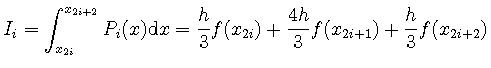
シンプソン法では, これら3点を通る2次式で関数を近似し, この2次式を積分する
ことで, この区間における積分値とする.
の3点を通る.
シンプソン法では, これら3点を通る2次式で関数を近似し, この2次式を積分する
ことで, この区間における積分値とする.
![\includegraphics[width=15cm]{numerical/simpson_model.eps}](img229.png)
この方法に従って実際に積分を求めてみる.
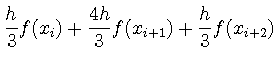
ここでは, 各区間の間隔を![]() とし,
とし,
![]() ,
, ![]() ,
, ![]() と置くことにする.
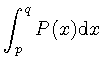
3点
と置くことにする.
3点 ![]() ,
, ![]() ,
, ![]() を通る2次曲線を
を通る2次曲線を![]() とすると,
とすると,
![]() は
は
 |
(51) |
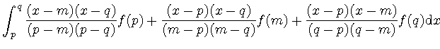
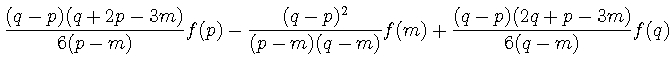
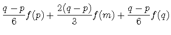
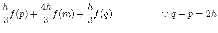
![]() であることに注意して,
であることに注意して,
![]() を
を![]() の領域で積分すると次のようになる.
の領域で積分すると次のようになる.
 |
(52) | ||
 |
(53) | ||
 |
(54) | ||
 |
(55) | ||
 |
(56) | ||
 |
(57) |
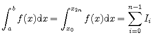
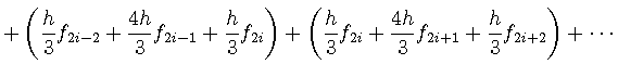
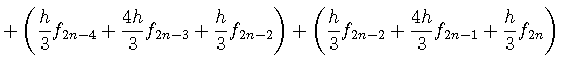
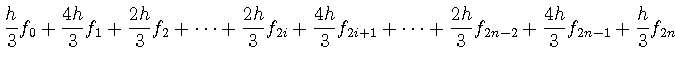
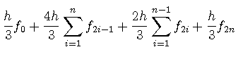
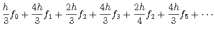
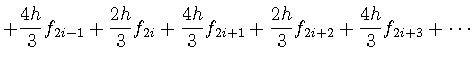
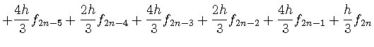
さらに, 次の図のように全積分領域![]() を
を![]() 等分し積分を考える.
ここで各区間の幅は
等分し積分を考える.
ここで各区間の幅は![]() である.
である.
![\includegraphics[width=20cm]{numerical/simpson_modelB.eps}](img230.png) 積分
積分
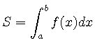 は,
は, ![]() と表記することにすると,
と表記することにすると,
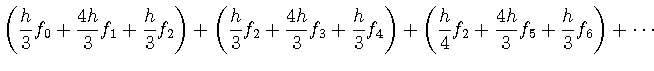
 |
(58) | ||
 |
(59) | ||
 |
(60) | ||
 |
(61) | ||
 |
(62) | ||
 |
(63) | ||
 |
(64) | ||
 |
(65) | ||
 |
(66) | ||
|
(67) | ||
|
(68) |
ここまででは, fprintf 関数によりファイルに出力することを行ってきた. ここでは, fscanf関数によりファイルから入力する.
fscanf関数 は以下の点で scanf 関数と異なるがそれ以外は同様に使用できる.
fscanf 関数
#include <stdio.h>
int fscanf(FILE *fp, const char *format, ...);
int  scanf(          const char *format, ...);
第2引数として, fscanf関数に予めオーブンしたファイルのファイルポインタを渡す. 第2引数として, fscanf 関数に与える書式 format は scanf 関数と共通. 第3引数以降には, 変数のアドレスを渡すことに注意.
以下に例を挙げる.
char c; int i; double x; char str[100]; double v[100]; // のとき

fscanf(fp, "%c",  &c);
fscanf(fp, "%d",  &i);
fscanf(fp, "%lf", &x); // double 型は "%lf". 間違え易いので注意.
fscanf(fp, "%s",  str);  // 文字列専用の書式として %s がある. str は char str[100] の先頭要素のアドレス.
fscanf(fp, "%lf", &v[2]); // 各要素に & を付けると, その要素のアドレス.

fscanf(fp, "%c%d%lf",  &c, &i, &x); // 複数の変数に入力
plot.cnfの内容の例:
red
5.0
4.2
plot.cnf の内容を変数に入力し, その値を画面に出力するプログラム:
#include <stdio.h>

int main(void)
{
	 FILE *fp;
	 char color[100];
	 double x, y;

	 if ( (fp=fopen("plot.cnf", "r")) == NULL ) {
		  printf("Can not open plot.cnf\n");
	 } else {
		  fscanf(fp, "%s", color);
		  fscanf(fp, "%lf", &x);
		  fscanf(fp, "%lf", &y);

		  printf("color=%s\n", color);
		  printf("x=%f\n", x);
		  printf("y=%f\n", y);

		  fclose(fp);
	 }

	 return 0;
}
gcc でコンパイルする場合は, svg1.h の中で数学関数を用いているので -lm オプションを付けておく.
$ emacs plot.cnf
$ emacs plot.c
$ gcc -Wall plot.c -lm
$ ./a.out
$ firefix drawing.svg
...                   # この後は コンパイルし直さなくても,
$ emacs plot.cnf      # plot.cnf を書き換え
$ ./a.out             # プログラムを実行すると
$ firefox drawing.svg # plot.cnf に応じて描画結果が変わっている.
【構造体の復習】
ATTRIBUTE circle_attrib;と宣言されている構造体のメンバーへの代入は, .を用いて circle_attrib.stroke = color;のように行う. ATTRIBUTE *circle_attrib;と構造体へのポインタとして宣言されているときは, 構造体のメンバーへの代入は, ->を用いてcircle_attrib->stroke = color;のように行う. (文法上は, ポインタとして宣言されている場合は (*circle_attrib).stroke = color; も正しい. ただし, この書き方は煩雑になることが多い思う.)
ATTRIBUTE circle_attrib;とATTRIBUTE *circle_attrib;は次のように使い分けるとよい. main関数などで, 実体を ATTRIBUTE circle_attrib;のようにして用意する. どこかで必ずこの実体の確保が必要である. 関数内で使用するときは, それへのポインタ(アドレス)を渡す. この場合呼び出される関数の仮引数は, ATTRIBUTE *circle_attrib となり, 関数内では ->を用いてメンバーを参照する.
【See also】
【実行の手順】
plot.c の内容:
#include <stdio.h>
#include <math.h>
#include "svg1.h"

int main(void)
{
	 FILE *fp;
	 char color[100];
	 double x, y;

	 // プロットに関係する変数.
	 SVG svg_file;
	 PLOT plot;
	 PLOT_VIEW view = {100.0, 50.0, 800.0, 500.0};
	 PLOT_WORLD world = {-10.0, -10.0, 10.0, 10.0};
	 PLOT_AXIS axis = {"x", 5, "y", 5};
	 ATTRIBUTE circle_attrib   = {"blue", 1.0, "white"};

	 // プロット初期化
	 plot_file_open(&svg_file, "drawing.svg", 855.0, 605.0);
	 plot_init(&plot, &svg_file, &view, &world, &axis);

	 if ( (fp=fopen("plot.cnf", "r")) == NULL ) {
		  printf("Can not open plot.cnf\n");
	 } else {
		  fscanf(fp, "%s", color);
		  fscanf(fp, "%lf", &x);
		  fscanf(fp, "%lf", &y);
		  circle_attrib.stroke = color;
		  plot_circle_draw(&plot, x, y, 5.0, &circle_attrib);
		  fclose(fp);
	 }

	 // プロット終了
	 plot_file_close(&plot);

	 return 0;
}
次のプログラムは, data.dat ファイルに記録されているデータを入力して, その値を画面に出力するプログラムである. fscanf 関数はファイルの最後まで入力が終了し次に入力する値が無いときに EOF を返す. EOF (End of File) は <stdio.h> の中で, 例えば #define EOF (-1)のように, 定義されている. 逆に, ファイル中から正しく入力が行われたときは, 入力された変数の数を返す.
このプログラムでは, fscanf 関数がEOFを返さない間, ファイルから入力を続ける. while の条件式の中で入力した xと y の値は, 条件が成立したとき実行するブロック内 ({ ... }) で使用できる. このプログラムでは, その値を画面に出力している.
このプログラムを実行する前に, 予め下に挙げる data.dat のようなデータファイルを作成しておくこと.
#include <stdio.h>

int main(void)
{
	 FILE *fp;
	 double x, y;

	 if ( (fp=fopen("data.dat", "r")) == NULL ) {
		  printf("Can not open plot.cnf\n");
	 } else {
		  while(fscanf(fp, "%lf%lf", &x, &y) != EOF){
			   printf("x=%f, y=%f\n", x, y);
		  }
		  fclose(fp);
	 }

	 return 0;
}
data.dat の内容の例:
0.7  5.0
3.8  6.4
5.8  5.7
8.4  5.2
9.3  3.0
13.1 3.8
13.2 6.6
ファイルから入力した値を画面に出力する代わりに, SVGファイルに描画するようにしたプログラムを示す.
#include <stdio.h>
#include <math.h>
#include "svg1.h"

int main(void)
{
	 FILE *fp;
	 double x, y;

	 // プロットに関係する変数.
	 SVG svg_file;
	 PLOT plot;
	 PLOT_VIEW view = {100.0, 50.0, 800.0, 500.0};
	 PLOT_WORLD world = {-5.0, -5.0, 20.0, 15.0};
	 PLOT_AXIS axis = {"x", 5, "y", 5};
	 ATTRIBUTE circle_attrib   = {"blue", 1.0, "white"};

	 // プロット初期化
	 plot_file_open(&svg_file, "drawing.svg", 855.0, 605.0);
	 plot_init(&plot, &svg_file, &view, &world, &axis);

	 if ( (fp=fopen("data.dat", "r")) == NULL ) {
		  printf("Can not open data.dat\n");
	 } else {
		  while(fscanf(fp, "%lf%lf", &x, &y) != EOF){
			   plot_circle_draw(&plot, x, y, 2.0, &circle_attrib);
		  }
		  fclose(fp);
	 }

	 // プロット終了
	 plot_file_close(&plot);

	 return 0;
}
描画結果が出力されている SVGファイル drawing.svg は, inkscape, Illustrator などで編集できるので試してみるとよい. inkscape で編集する場合は, 予め $ inkscape &のように起動しておき, File メニューから Open する. もしくは, ファイルブラウザ (nautilus) を起動して, 編集したいファイルを inkscape にドラッグする. (本来 $ inkscape drawing.svg & のようにファイル名を指定して起動できますが, 全学計算機システムでは設定がうまくいっていないようです.)
CSV ファイルは, コンマで各フィールドを区切ったデータファイルである. たとえば 次のような内容を持つ. これをfscanf で入力するときは, "%lf,%lf" のように書式に ,(コンマ)を入れおく.
data.csv の内容の例:
0.7,  5.0
3.8,  6.4
5.8,  5.7
8.4,  5.2
9.3,  3.0
13.1, 3.8
13.2, 6.6
#include <stdio.h>

int main(void)
{
	 FILE *fp;
	 double x, y;

	 if ( (fp=fopen("data.csv", "r")) == NULL ) {
		  printf("Can not open plot.cnf\n");
	 } else {
		  while(fscanf(fp, "%lf, %lf", &x, &y) != EOF){
			   printf("x=%f, y=%f\n", x, y);
		  }
		  fclose(fp);
	 }

	 return 0;
}
CSVファイルには, 次に挙げるようにテキストのフィールドは "で囲んだ上で, コンマで区切るものもある. 上のプログラムでは入力できないので修正する必要がある.
"x", "y"
0.7,  5.0
3.8,  6.4
5.8,  5.7
8.4,  5.2
9.3,  3.0
13.1, 3.8
13.2, 6.6
要望があれば続きを書きます...
(c)1999-2013 Tetsuya Makimura
![\includegraphics[width=15cm]{numerical/daikei.eps}](img165.png)